Journal Club for Analysis of Complex Datasets
- Sebastiani et al, Nature Genetics 37:435;2005: Genetic dissection and prognostic modeling of overt stroke in sickle cell anemia.
- Lewin et al (2006), Biometrics 62(2):1-9: Bayesian modeling of differential gene expression; Gottardo et al (2006), Biometrics 62(2):10-18: Bayesian robust inference for differential gene expression in microarray with multiple samples.
- Richard Simon, Roadmap for Developing and Validating Therapeutically Relevant Genomic Classifiers, Journal of Clinical Oncology, Vol 23, No 29 (October 10), 2005: pp. 7332-7341. Richard Simon, Michael D. Radmacher, Kevin Dobbin, Lisa M. McShane, Pitfalls in the Use of DNA Microarray Data for Diagnostic and Prognostic Classification, J Natl Cancer Inst 2003; 95: 14-18
- Raghavan et al. On Methods for Gene Function Scoring as a Means of Facilitating the Interpretation of Microarray Results. Journal of Computational Biology, 13(3): 798-809, 2006.
- Dupuy A, Simon RM, Critical Review of Published Microarray Studies for Cancer Outcome and Guidelines on Statistical Analysis and Reporting, J Natl Cancer Inst 2007;99:147-157
- Zhang et al. Prospective Cohort Study of soy Food Consumption and Risk of Bone Fracture among Postmenopausal Women, Arch Intern Med. 2005;165:1890-1895. Cui et al. Association of Ginseng Use with Survival and Quality of Life among Breast Cancer Patients, Am J Epidemiol 2006;163:645-653.
- Frost et al. Influenza and COPD mortality protection as pleiotropic, dose-dependent effects of statins, Chest. 2007; 131: 1006-1012.
- Bovelstad, Nygard, Storvold, et al: Predicting survival from microarray data - a comparative study. Bioinformatics 23:2080-2087; 2007.
- Lee et al, An extensive comparison of recent classification tools applied to microarray data. Computational Statistics & Data Analysis 48 (2005) 869-885
Sebastiani et al, Nature Genetics 37:435;2005: Genetic dissection and prognostic modeling of overt stroke in sickle cell anemia.
- Full Text | Commentary | Supplemental Information
- 18 Apr 2006, noon-1pm, Room D-2221 Med Ctr North, RSVP to biostat@vanderbilt.edu
- Discussed by FrankHarrell and ConstantinAliferis
Goals and Data
- Find persons with sickle cell anemia at risk of overt stroke (6-8% incidence)
- Genetic dissection: disentangling interactions among genes, environment, phenotype
- 108 SNPs in 80 (?39) candidate genes
- Unspecified extensive clinical variables also used
- 1398 African Americans with SCA, 92 strokes
Pattern Recognition using Bayesian Network | Aliferis Commentary
- Focused on networks describing dependencies of genotypes on phenotype
- Authors state that strategy is more diagnostic than prognostic
- Did not take variable follow-up into account
- Used Bayesware Discoverer which claims to do "automated discovery of Bayesian networks from data"
- $5,500 for one user license; first 2 authors are owners; not open source
- Found that 31 SNPs in 12 genes interact with fetal hemoglobin to predict stroke risk
- Final network had 73 nodes (fig. 2, 69 SNPs, avg. 1.3 strokes per node)
- "the model is able to describe the determinant effects of genetic variants on stroke"
- Stability benefits from smart choices of candidate genes
- Bayes factor of
 quantifying the relative likelihood that a SNP is associated with stroke vs. being independent may be problematic
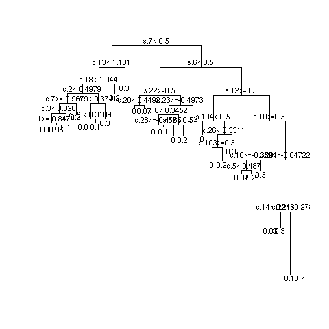
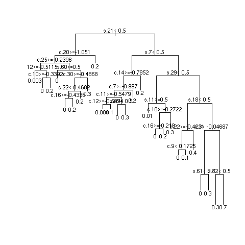
- BN is not dissimilar to tree modeling using recursive partitioning
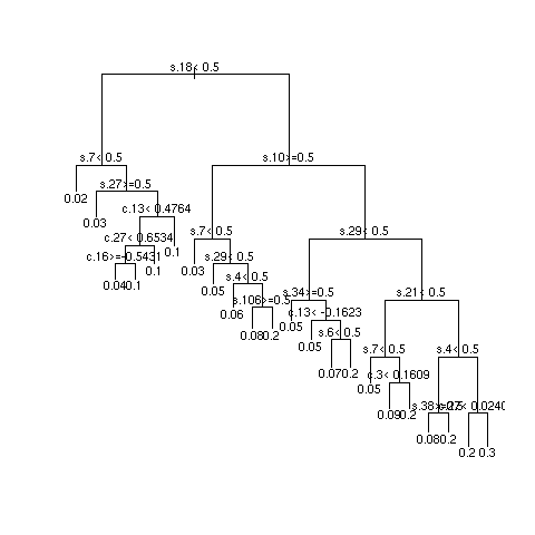
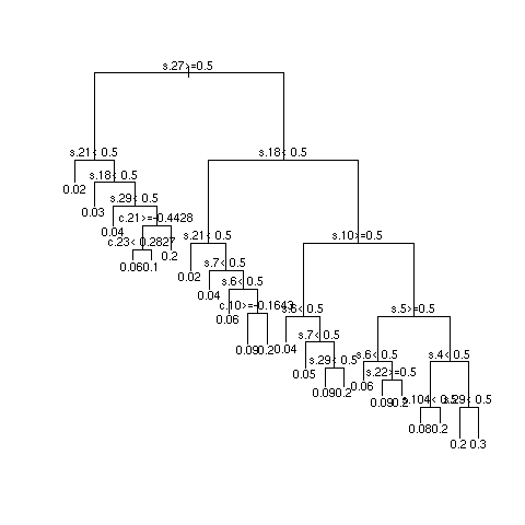
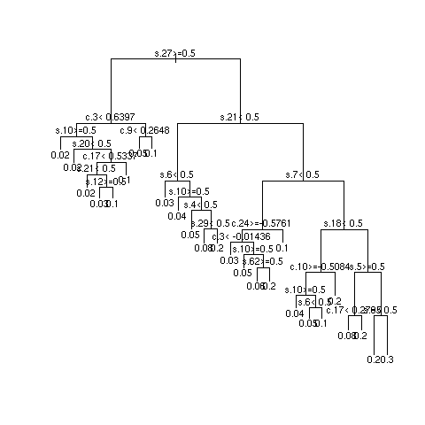
- Example simulations showing instability
- Simulated data from additive logistic model with sample size of 1490 patients having a target of 92 strokes
- 108 SNPs (binary, prevalence 0.5) having importance (weights) shown below
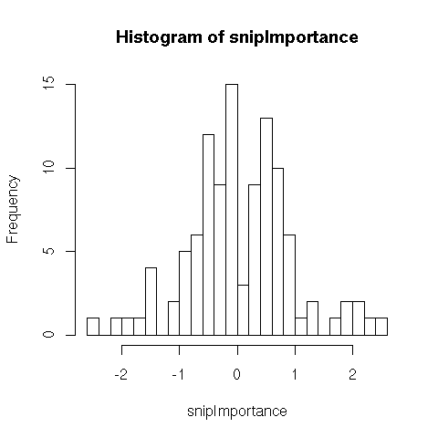
- 30 clinical variables (normal with mean 0 and standard deviation .5), weights uniform between -1 and 1
- 3 independent repetitions of recursive partitional
- Most important SNPs: s18 and s27; most important clinical variables: c13 and c8
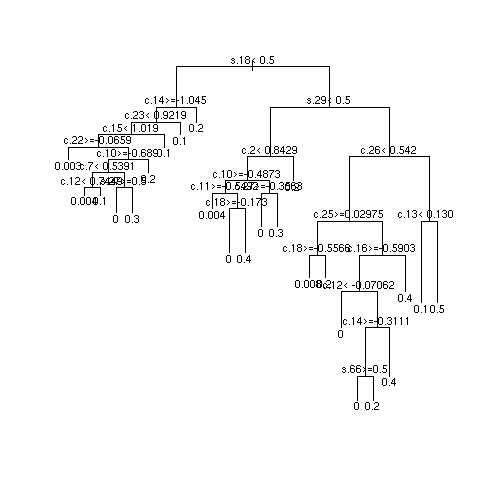
- Multiply sample size by 10 and repeat
Quantifying Predictive Accuracy
- Proportional classified correctly is an improper scoring rule (optimized by a miscalibrated model)
- Arbitrary and covers up "gray zone" (authors used cutoff of 0.5 risk)
- Loss of statistical power
- Authors did independent validation on 114 patients (7 with stroke), got 98.2% correct (112/114, predicted all strokes correctly, predicted 2 strokes in patients without stroke)
- Fig. 3 treats stroke as the predictor and the probability of stroke as the response variable
- Need a calibration plot
- Authors gave no confidence limits on their validated proportion correct [0.938, 0.995] but will the classification rule transport?
- Need a more continuous measure of discrimination ability that does not require arbitrary classification
- Area under ROC curve (C-index), Brier score
Difficulty in Estimating Accuracy in Small Samples
The following plot shows the results of a simulation of an ever-increasing test sample used to validate the most simple (and inappropriate) accuracy measure, the proportion classified correctly, when the true proportion is 0.8. This is also the least stringent validation, because if the outcome incidence is 0.2, one would be 0.8 accurate just by predicting that no patient will suffer the event. Validations need to be 2-sided (e.g., false positive and false negative rates) or a better measure such as overall calibration accuracy should be used. Outer bands are 0.95 confidence intervals for the presumably unknown true probability of correct prediction.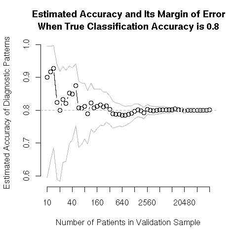
Commentary
- Meschia and Pankratz (p. 340-1): "Despite their promise, it is important to temper enthusiasm for Bayesian networks and similar analytical techniques. Results from these analytical techniques are dependent on the structure of the model, and their statistical properties have not yet been fully studied. The complex data analaytical techniques that can be applied to large data sets make it possible to obtain persuasive results for any given data set. If nuances in sample set identification, data collection and application of the method are overlooked, then the results that are obtained may be difficult to replicate, or even misleading. ... we recommend that extensive detail be provided about every component of the study design and analysis, including a detailed description of the intermediate steps in model creation."
Lewin et al (2006), Biometrics 62(2):1-9: Bayesian modeling of differential gene expression; Gottardo et al (2006), Biometrics 62(2):10-18: Bayesian robust inference for differential gene expression in microarray with multiple samples.
- Full Text for Lewin et al | Supplemental Information | Full Text for Gottado et al
- 2 May 2006, noon-1pm, Room D-2221 MCN, RSVP to biostat@vanderbilt.edu
- Discussed by Chuan Zhou and Frank Harrell
- Discussion Slides
Richard Simon, Roadmap for Developing and Validating Therapeutically Relevant Genomic Classifiers, Journal of Clinical Oncology, Vol 23, No 29 (October 10), 2005: pp. 7332-7341. Richard Simon, Michael D. Radmacher, Kevin Dobbin, Lisa M. McShane, Pitfalls in the Use of DNA Microarray Data for Diagnostic and Prognostic Classification, J Natl Cancer Inst 2003; 95: 14-18
- Full Text for Simon paper 1 | Full Text for Simon paper 2
- 25 July 2006, noon-1pm, Room D-2221 MCN, RSVP to biostat@vanderbilt.edu
- Discussed by Deming Mi and Frank Harrell
Raghavan et al. On Methods for Gene Function Scoring as a Means of Facilitating the Interpretation of Microarray Results. Journal of Computational Biology, 13(3): 798-809, 2006.
Basic information
- http://www.ncbi.nlm.nih.gov/entrez/query.fcgi?cmd=Retrieve&db=PubMed&list_uids=16706726 Entrez PubMed Link
- Full Text Link
- 15 August 2006, noon-1pm, Room D-2221 MCN, RSVP to biostat@vanderbilt.edu
- Discussed by Bing Zhang and Lily Wang
Outline of the discussion
- Motivation: Interpretation the results from microarray experiments is nontrivial. Integration of gene function or pathway information into the analysis should allow better understanding of the molecular mechanisms. A few methods have been proposed without performance assessment. This paper will compare various existing and new methods on this topic.
- Introduction to gene function and pathway information resources
- Test statistics (Overrepresentation analysis, functional class scoring, distributional scores), their pros and cons
- Resampling schemes
- Calibration of critical values based on the size of gene categories
- Results from the paper based on both simulation and real data
- Remaining questions
Dupuy A, Simon RM, Critical Review of Published Microarray Studies for Cancer Outcome and Guidelines on Statistical Analysis and Reporting, J Natl Cancer Inst 2007;99:147-157
Basic Information
- 6 Feb 2007, noon-1pm, Room D-2221 MCN, RSVP to biostat@vanderbilt.edu
- Discussed by Constantin Aliferis and Lily Wang
- Full text
Outline of the Discussion
- Systematic review of gene expression microarray studies for cancer outcome
- Common flaws in data analysis (with comments)
- Guidelines for statistical analysis and reporting
Zhang et al. Prospective Cohort Study of soy Food Consumption and Risk of Bone Fracture among Postmenopausal Women, Arch Intern Med. 2005;165:1890-1895. Cui et al. Association of Ginseng Use with Survival and Quality of Life among Breast Cancer Patients, Am J Epidemiol 2006;163:645-653.
Basic Information
- 20 March 2007, noon-1pm, Room D-2221 MCN, RSVP to biostat@vanderbilt.edu
- Discussed by Chuan Zhou, Patrick Arbogast, and Robert Greevy
- Soy paper
- Ginseng paper
Outline of the Discussion
- Pros and cons of cohort studies
- Association vs. causality
- Propensity score and related methods
- Discussion slides
- journal_club_2007mar20_ginseng_breast_cancer_survival_QOL.ppt:
- soydiscuss-032007.pdf:
Frost et al. Influenza and COPD mortality protection as pleiotropic, dose-dependent effects of statins, Chest. 2007; 131: 1006-1012.
Basic Information
- 22 May 2007, noon-1pm, Room D-2221 MCN, RSVP to biostat@vanderbilt.edu
- Discussed by Patrick Arbogast, and Ayumi Shintani
- http://www.chestjournal.org/cgi/reprint/131/4/1006.pdf
Outline of the Discussion
- Immortal time bias
- Unmeasured confounders
- Choice of regression models
- Discussion slides
- journal_club_2007may22_influenza_copd_statins.ppt:
Bovelstad, Nygard, Storvold, et al: Predicting survival from microarray data - a comparative study. Bioinformatics 23:2080-2087; 2007.
- The paper has much to offer
- Need to explore the following to add to the results: adaptive lasso, pre-conditioning, sparse principal components, elastic net
- Related to sparce PC, the authors may not have used Tibshirani's R algorithm
Lee et al, An extensive comparison of recent classification tools applied to microarray data. Computational Statistics & Data Analysis 48 (2005) 869-885
- Recent Classification Tools
- 30 Mar 2010, noon-1pm, Room D-2221 Med Ctr North
- Discussed by Vincent Agboto, Ph.D.


This topic: Main > WebHome > Clinics > ClinicOmics > ComplexDataJournalClub
Topic revision: revision 36
Topic revision: revision 36
Ideas, requests, problems regarding Vanderbilt Biostatistics Wiki? Send feedback