Mid-term Exam

Due 13Mar08 9am in S-2323 Medical Center North or e-mailed to the grading assistant

This exam is to be taken under conditions given by the Vanderbilt honor code. Do not ask for help for questions from anyone except the instructors. We will reply through the discussion board so everyone has the opportunity to benefit equally from our responses.

Problem 1

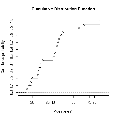
A study has collected ages in a random sample from a population. Consider the empirical cumulative distribution of ages (Figure 1) and the frequency distribution (Figure 2) to answer the following questions.

1. What is the estimated probability that age is less than or equal to 35 years?
2. What is the estimated probability that age is greater than 75 years?
3. What is the estimated probability that age is between 35 and 60 years?
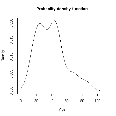
4. Describe the shape of the distribution of age using the provided empirical CDF or the probability density (frequency distribution)
   

Note that there are 20 subjects in the sample, so each of your answers to 1, 2, and 3 should be divisible by 0.05 (e.g. 0.05, 0.10, 0.15, etc)

• Figure 1. Empirical Cumulative Distribution Function (Problem 1):
  

• Figure 2. Probability Density Function (Problem 1):
  

Problem 2

Investigators are interested in determining if tumor volume at 5 weeks is different in a group of mice receiving a treatment (group 1) compared to a group of mice receiving a placebo (group 2). In 10 mice receiving the treatment, they calculate and and in 13 mice receiving a placebo, .

1. State the null and alternative hypotheses for a two-sample t-test of this research question. Use and to represent the population means in group 1 and group 2, respectively.
2. Carry out the two sample t-test (equal variances) being sure to indicate (a) the pooled estimate of the variance, (b) the test statistic (T), and (c) p-value.
3. Based on your results in part 2, do you reject or fail to reject H0 at a significance level of 0.01? State your scientific conclusions using terminology that the investigator (a non-statistician) can understand.
4. Calculate a 99% confidence interval for , the difference in population means
5. What are the assumptions of the 2-sample t-test that need to be satisfied for this test to be valid? Explain how you would verify these assumptions. With the given sample means and standard deviations, is there any indication that one or more of these assumptions may not hold?

Problem 3

Researchers were interested in estimating the average fetal head circumference at 20 weeks gestation. In a sample of n = 10 subjects, they found = 3.70 and s = 1.17. Head circumference is assumed to follow a normal distribution, so they calculated a 95% CI for the population mean head circumference to be [2.86, 4.53]. The width of this confidence interval is defined to be the upper limit (4.53) minus the lower limit (2.86), which is 1.67. For each of the following situations, indicate if the width of the confidence interval will increase, decrease, or remain the same if the stated parameter is changed while the other paramters are held constant. Briefly explain your reasoning.

1. The significance level, alpha, is increased
2. The sample size, n, is increased
3. The sample standard deviation, s, increases
4. If we assume the standard deviation () is known, and = s
5. increases (s remains at 1.17)

Problem 4

Consider the hematologic data for patients with aplastic anemia B Rosner Fundamentals of Biostatistics, 5th Edition (Duxbury, Pacific Grove CA), 2000, p. 503.

Patient	% reticulytes	Lymphocytes
number		(per mm2)
1	3.6	1700
2	2.0	3078
3	0.3	1820
4	0.3	2706
5	0.2	2086
6	3.0	2299
7	0.0	676
8	1.0	2088
9	2.2	2013

1. Fit a regression line relating the percentage of reticulytes (x) to the number of lymphocytes (y)
2. Test for the statistical significance of this regression line using the F-test.
3. What is for this problem and what is its interpretation?
4. What is the value of and what is its interpretation?
5. Test for the statistical significance of the regression line using the t test.
6. What are the standard errors of the slope and intercept for the regression line?
7. Obtain an approximate 0.95 confidence interval for the population slope, then obtain an exact confidence interval, both assuming normality and constant variance of the residuals.
8. Estimate E(lymphocytes | % reticulytes=3) and compute 0.95 confidence intervals for this expected (mean) value
9. Estimate the lymphocyte count for an individual with 3% reticulytes and compute 0.95 confidence limits corresponding to this individual's estimate
10. Estimate the conditional (the standard deviation of lymphocytes across patients with the same % reticulytes)

Problem 5

Consider Rosner's lead dataset we have been analyzing in class. Perform a more thorough analysis.

1. Considering the response variable maxfwt and predictor variables age and sex, create appropriate graphics (not model fits) to explore the relationship between age, sex, and the dependent variable maxfwt. Include raw data and smooth trend lines where appropriate.
2. Fit a linear model with the predictors age, sex, group. Allow the slope for age to vary with sex. Precisely interpret the estimated regression coefficients (including the intercept) and compute and interpret the overall . Interpret the t statistic for the age x sex effect.
3. Fit a new model containing only the continuous lead levels in 1972 and 1973 as the two predictors (not dichotomized arbitrarily as we have been doing). Interpret coefficient estimates and . Use t-tests to assess whether each of the lead levels is needed in predicting maxfwt once the other lead level is adjusted for. What is the weighted combination of lead levels that best predicts maxfwt?
4. To the two lead levels add age and sex. Interpret the increase in and obtain the SSR due to the combination of the two lead levels. Obtain a partial F-test to test whether either of the two lead levels is associated with maxfwt after adjusting for age and sex.
5. Add the following predictors to the four used in the last model: distance from the smelting plant and number of years spent within 4.1 miles of the plant (assume linearity of effect of this variable). Obtain partial SSRs and F-tests for the two lead levels (2 numerator d.f.). Comment on any differences you observe in these partial (adjusted) statistics between this full adjustment and the less comprehensive model that used only the four variables.
6. Using only one statistic, test whether any of the exposure-related risk factors is associated with maxfwt after adjusting for the effects of age and sex. Describe how the numerator degrees of freedom in the F-statistic arose.