Exploring RGB Colorspace with R
I've recently been exploring the
DataExpo2006 data set, and it got me thinking
about using color gradients in graphs. Actually, I showed some folks here around the office some of my graphs, and someone asked how I arrived at the color schemes.
I told him that I used the
RColorBrewer package that implements the
ColorBrewer 1 color schemes. He asked why I didn't just create the schemes myself automatically, and how
did I know the ColorBrewer schemes were good...
There's always someone.
I could have said I don't care if they're good or not and that the colors
look fine to me, but I thought I should at least try to find out the how and the
why. It turns out that Cynthia Brewer, the Brewer in ColorBrewer and a professor of Geography, has done quite a bit of work to get color schemes that look good on your computer screen to also look
good when you use them in production quality prints of maps, which is a huge pain. She arrived at her schemes not through following arcs through a colorspace, nor by creating perceptually equal color steps, both algorithmic processes, but by design. I don't know exactly what that means yet (I'll let you know when I find out), but I presume
it meant that she used her artistic intuition, a subjective process... But she does have a
Fine Arts degree with distinction.
But this note wasn't meant to be about Cynthia nor ColorBrewer; it's actually about the following graphs.
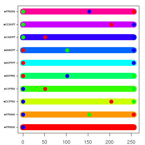
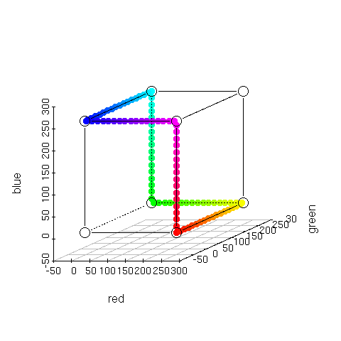
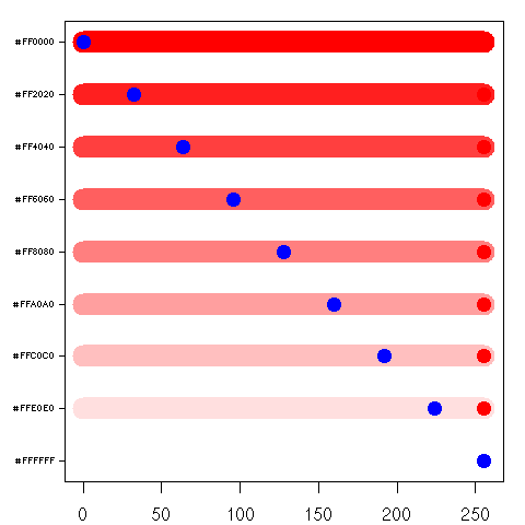
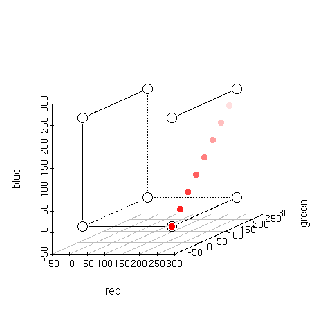
I wanted to get a handle on what those Red, Green, and Blue values looked like with the set (or scheme) of colors they created, so I devised the following plot (it utilizes Paul Murrell's venerable grid package). The X axis ranges from 0 to 255 and notes the Red, Green, and Blue values. The Y axis is the set of colors; the Y label giving the hex triplet for that particular color. For each color I plot, I also plot the Red, Green, and Blue component on top of the color. Below, the plots on the left are the ones I devised, while the plots on the right are views in 3d rgb colorspace using Uwe Ligges'
scatterplot3d package. I also created an mpeg movie with scatterplot3d varying the angle from 1 to 180. Here's all the
R code. I think the resulting plots are interesting.
| > plotcol2d(rainbow(10)) |
> plotcol3d(rainbow(10),angle=24) |
 |

Download Movie |
A plot of 10 of the colors returned by the R function
rainbow(). Nothing really interesting here, except that some of the Red, Green, and Blue dots are obscured. This happens for a couple of reasons:
- 1) the order in which the dots are drawn is red first, green second, blue third, and if any have the same value, then they will be obscured.
- 2) the color itself may partially or fully obscure one of the dots.
This is okay, since you can compute the independent components from the hexadecimal encoded color label: Red first, Green second, and Blue third. For instance, the second color from the bottom up "#FF9900" represents the Red component at 255, Green at 153, and Blue at 0.
| > plotcol2d(rainbow(100)) |
> plotcol3d(rainbow(100),angle=24) |
 |
Download Movie |
Plot of 100 of the
rainbow() colors. Quite nice. Now that I'm plotting so many colors, a gradient effect occurs, and some of the color labels are obscured. You can also see how the colors travel through 3d colorspace.
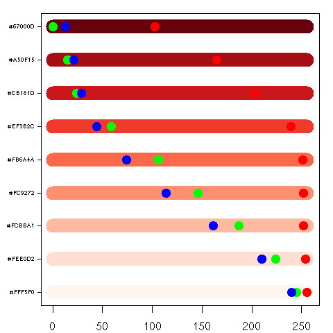
| > plotcol2d(brewer.pal(9,'Reds')) |
> plotcol3d(brewer.pal(9,'Reds'),angle=24) |
 |
Download Movie |
Here's Brewer's Red sequential color scheme. Notice how each color (she refers to them as classes) in the scheme is different.
Compare this to the following plots.
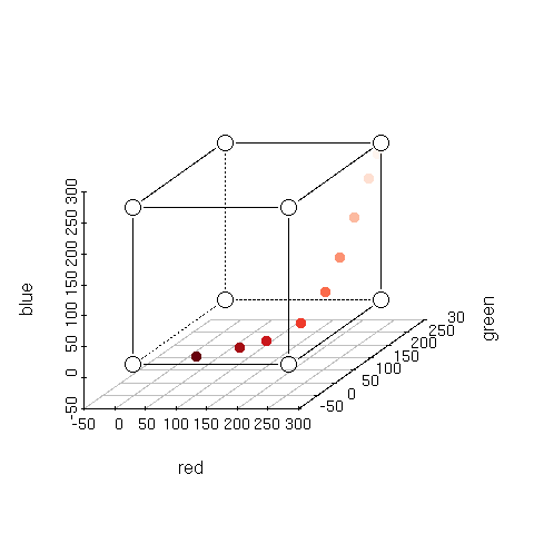
> plotcol2d(
rev(
rgb(255,
ceiling(seq(0,255,len=9)),
ceiling(seq(0,255,len=9)),max=255))) |
> plotcol3d(
rev(
rgb(255,
ceiling(seq(0,255,len=9)),
ceiling(seq(0,255,len=9)),max=255)),angle=24) |
 |
Download Movie |
Red stays constant at 255 while Green and Blue decrease from 255 to 0 in 9 steps. Notice
how the top three colors are almost identical. You would certainly want to use Brewer's Reds over these if you wanted 9 perceptually different colors.
R Source Code
In addition to the plotcol2d() code and plotcol3d(), there's extra code for matrix rotation and linear interpolation in both directions. These are useful for extending color schemes like
Brewer's that only contain a small number of colors.
library(grid)
library(RColorBrewer)
library(scatterplot3d)
# Rotate a matrix 90deg clockwise
rot90 <- function(mat) t(mat[nrow(mat):1,])
# Rotate a matrix 90deg counterclockwise
rotn90 <- function(mat) t(mat[,ncol(mat):1])
# Arbitrary rotation of a matrix in either direction
# mat - matrix to rotate
# deg - A positive deg rotates clockwise, negative counterclockwise
#
# returns the rotated matrix
mat.rot <- function(mat,deg){
# the modulus %% operator does the right thing with negative degrees
# thus -90 %% 360 == 270
ndeg = deg %% 360
if (ndeg==90)
return(rot90(mat))
if (ndeg==180)
return(rot90(rot90(mat)))
if (ndeg==270)
return(rotn90(mat))
mat
}
# Function for linearly interpolating a matrix in the x (row) dimension
# mat - the matrix to interpolate
# ixdim - the dimension
#
# returns interpolated matrix in x dimension
mat.interp.x <- function(mat,ixdim){
xdim <- dim(mat)[1]
ydim <- dim(mat)[2]
if (is.na(ixdim) && (ixdim-xdim)>0){
z <- matrix(nrow=ixdim,ncol=ydim)
for (i in 1:ydim){
z[,i] <- approx(1:xdim,mat[,i],n=ixdim)$y
}
return(z)
}
mat
}
# Function for interpolating a matrix in the x (row) or y (col) dimension
# mat - the matrix to interpolate
# ix - the x dimension to grow to. If set to NA, then keep same x dimension
# iy - the y dimension to grow to. If set to NA, then keep same y dimension
#
# returns interpolated matrix
mat.interp <- function(mat,ix,iy){
mdim <- dim(mat)
# try and interpolate in x direction
if (is.na(ix)){
if ((ix-mdim[1])<=0){
warning(sprintf("x dimension is too small: %d<=%d",mdim[1],ix))
return(mat)
}
newmat <- mat.interp.x(mat,ix)
mdim <- dim(mat)
} else {
newmat <- mat
}
if (is.na(iy)){
if ((iy-mdim[2])<=0){
warning(sprintf("y dimension is too small: %d<=%d",mdim[2],iy))
return(mat)
}
newmat <- mat.rot(mat.interp.x(mat.rot(newmat,90),iy),-90)
}
newmat
}
plotcol2d <- function(cols){
x <- 1:255
y <- 1:length(cols)
pushViewport(plotViewport(c(5.1,4.1,4.1,2.1)))
pushViewport(dataViewport(x,y))
grid.rect()
grid.yaxis(y,label=cols,gp=gpar(fontsize=6))
grid.xaxis()
red = col2rgb(cols)[1,]
green = col2rgb(cols)[2,]
blue = col2rgb(cols)[3,]
for (i in y){
grid.lines(c(0,255),i,default.units="native",gp=gpar(col=cols[i],lwd=20),draw=TRUE)
}
grid.points(red,y,pch=16,gp=gpar(col="red"),draw=TRUE)
grid.points(green,y,pch=16,gp=gpar(col="green"),draw=TRUE)
grid.points(blue,y,pch=16,gp=gpar(col="blue"),draw=TRUE)
popViewport(2)
}
# Extends the range of colors in cols by linearly interpolating the red, green, and
# blue components.
extend.colrange <- function (cols,n){
c <- floor(mat.interp(col2rgb(cols),NA,n))
rgb(c[1,],c[2,],c[3,],max=255)
}
# Apply a function over cols
# for instance "fun=function(x) length(x)/log(length(x)) * log(x)"
scale.cols <- function(cols,fun=function(x){x}){
x <- 1:length(cols)
y <- ceiling(fun(x))
for (i in x){
if (is.na(y[i])) y[i] <- 1
if (y[i] < 1) y[i] <- 1
if (y[i] > length(y)) y[i] <- length(y)
}
cols[y]
}
# From scatterplot3d() R help file
cubedraw <- function(res3d, min = 0, max = 255, cex = 2, text. = FALSE) {
## Purpose: Draw nice cube with corners
cube01 <- rbind(c(0,0,1), 0, c(1,0,0), c(1,1,0), 1, c(0,1,1), # < 6 outer
c(1,0,1), c(0,1,0)) # <- "inner": fore- & back-ground
cub <- min + (max-min)* cube01
## visibile corners + lines:
res3d$points3d(cub[c(1:6,1,7,3,7,5) ,], cex = cex, type = 'b', lty = 1)
## hidden corner + lines
res3d$points3d(cub[c(2,8,4,8,6), ], cex = cex, type = 'b', lty = 3)
if(text.)## debug
text(res3d$xyz.convert(cub), labels=1:nrow(cub), col='tomato', cex=2)
}
plotcol3d <- function(cols,angle=1){
cm <- t(col2rgb(cols))
p <- scatterplot3d(cm,color=cols, box = FALSE, angle = angle,
xlim = c(-50, 300), ylim = c(-50, 300), zlim = c(-50, 300))
p$points3d(cm,col=cols,pch=16)
cubedraw(p)
}
mov.plotcol3d <- function(cols,dir){
for (i in 1:180){
file <- sprintf('%s/plotcol3d%03d.png',dir,i)
png(filename=file)
plotcol3d(cols,i)
dev.off()
}
}
make.mov.plotcol3d <- function(){
unlink("plotcol3d.mpg")
system("convert -delay 10 plotcol3d*.png plotcol3d.mpg")
}