
You are here: Vanderbilt Biostatistics Wiki>Main Web>TatsukiRcode (16 Jul 2024, TatsukiKoyama)Edit Attach
R code for tplot, kmplot and other functions.
- RFunctions1.R: RFunctions1.R
R code for other miscellaneous functions.
- RFunctions2.R: RFunctions2.R
R code for simulating 3+3 designs.
- Three3.R: Three3.R
R code for inference from two-stage adaptive design
- Koyama T and Chen H. ``Proper inference from Simon's two-stage designs'' Statistics in Medicine 27(16), 2008. PMID: 17960777. PMCID: PMC6047527.
- The main page
- twostage2020Web.R: R code: Inference from two-stage designs
R code for confidence intervals on micro-averaged F1 and macro-averaged F1 scores
- Takahashi K, Yamamoto K, Kuchiba A, Koyama T. Confidence interval for micro-averaged F (1) and macro-averaged F (1) scores. Appl Intell (Dordr). 2022 Mar;52(5):4961-4972. doi: 10.1007/s10489-021-02635-5. Epub 2021 Jul 31.
- f1Scores.R: R code: Confidence intervals for F1 scores
R code for the Length of the Beatles' Songs plot
kmplot() tplot() jmplot() dsplot() showcolors()
kmplot()
- Kaplan-Meier survival plot with at-risk table
- plot Kaplan-Meier curves with 'numbers at risk' at bottom margin.
- can specify at which time n at-risk is displayed
- can specify line type / line width / line color for each line
- can change the order of appearance in the n at-risk table
- n.at.risk numbers are right-justified!
- simple=TRUE suppresses the 'at risk' table.
Example
require(survival)
kma <- survfit( Surv(time, status) ~ rx + adhere, data=colon )


kmplot(kma, mark='', simple=FALSE,
	xaxis.at=c(0,.5,1:9)*365, xaxis.lab=c(0,.5,1:9), # n.risk.at
	lty.surv=c(1,2), lwd.surv=1, col.surv=c(1,1,2,2,4,4), # survival.curves
	col.ci=0, # confidence intervals not plotted
	group.names=c('Obs ','Obs tumor adh','Lev','Lev tumor adh','Lev+5FU ','Lev+5FU tumor adh'),
	group.order=c(5,3,1,6,4,2), # order of appearance in the n.risk.at table and legend.
	extra.left.margin=6, label.n.at.risk=FALSE, draw.lines=TRUE,
	cex.axis=.8, xlab='Years', ylab='Survival Probability', # labels
	grid=TRUE, lty.grid=1, lwd.grid=1, col.grid=grey(.9),
	legend=TRUE, loc.legend='bottomleft',
	cex.lab=.8, xaxs='r', bty='L', las=1, tcl=-.2  # other parameters passed to plot()
)
title(main='Chemotherapy for stage B/C colon cancer', adj=.1, font.main=1, line=0.5, cex.main=1)

tplot()
tplot() is an alternative to boxplot(). The individual data can be shown (either in the foreground or background) with jittering if necessary.Example
This example shows what options are available with tplot(). This may not be a good way to show these data (unnecessary color varieties...)col and pch may be specified at the individual level or group level. (In this example, col is specified at the individual level, and pch is specified for groups.)
colors of boxes and box borders are specified by boxcol and boxborder.
boxplot.pars is passed to boxplot().
set.seed(100)
age <- rnorm(80, rep(c(26,36), c(70,10)), 4)
sex <- factor( sample(c('Female','Male'), 80, TRUE) )
group <- paste('Group ', sample(1:4, 40, prob=c(2,5,4,1), replace=TRUE), sep='')
d <- data.frame(age, sex, group)

tplot( age ~ group, data=d,
    las=1, cex=1, cex.axis=1, bty='L',
    show.n=TRUE, dist=.25, jit=.05, type=c('db','db','db','d'),
    group.pch=TRUE, pch=c(15,17,19,8),
    col=c('darkred','darkblue')[c(sex)],
    boxcol=c('lightsteelblue1','lightyellow1',grey(.9), 0), boxborder=grey(.8),
    boxplot.pars=list(notch=TRUE, boxwex=.5)
    )

jmplot()
- Joint distribution and marginal distributions on its margins.
- requires tplot() [See above.]
Example
 set.seed(274)
 x <- rnorm(100, 20, 5)
 y <- rexp(100)
 levels <- as.factor(sample(c("Male","Female"), 100, TRUE))
 jmplot(x, y, levels, col=levels, las=1, type='db', main='Some scores', jit=.02)

dsplot()
- Discrete Scatter Plot for Integer-valued variables
- This creates a scatter plot (sort of) for discrete bivariate data. An alternative to sunflower plots.
Example
set.seed(6)
x <- round(rnorm(400, 100, 4))
y <- round(rnorm(400, 200, 4))
sex <- sample(c('Female','Male'), 400, T)
dsplot(y ~ x, pch=19, col=1+(sex=='Female'), cex=.6, bkgr=T,
   xlab='measurement 1', ylab='measurement 2', bty='L')
legend( 'bottomright', pch=19, col=1:2, legend=c('Male','Female'), cex=.8 )

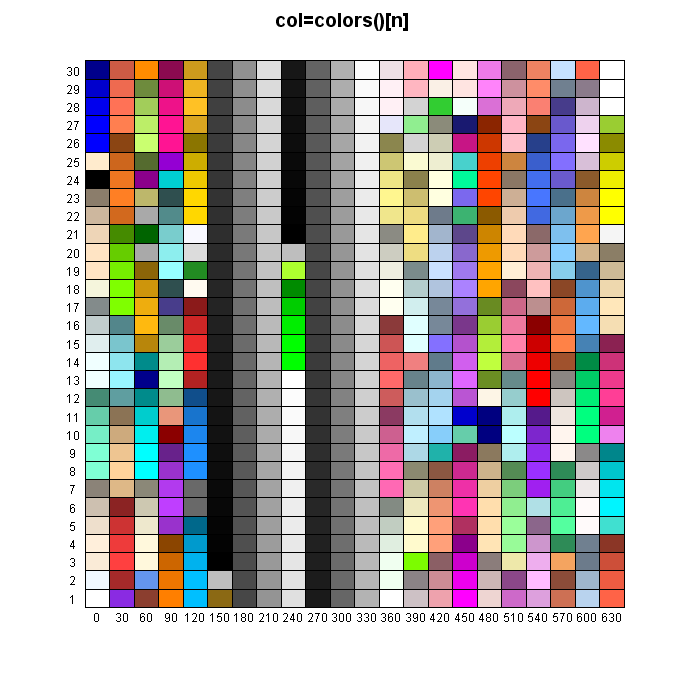
Show colors
In R, there are 657 named colors. The following funciton, show.colors(), shows these colors and corresponding numbers.
Find the color you like in the plot. You can find the name of the color by running >colors()[number].
show.colors <- function(){
   par(mfrow=c(1,1))
   #   par(mai=c(.4,.4,.4,.4), oma=c(.2,0,0,.2))
   x <- 22 ; y <- 30
   plot(c(-1,x),c(-1,y), xlab='', ylab='', type='n', xaxt='n', yaxt='n', bty='n')
   for(i in 1:x){for(j in 1:y){
         k <- y*(i-1)+j ; co <- colors()[k]
         rect(i-1, j-1, i, j, col=co, border=grey(.5) )}}


   text(rep(-.5,y),(1:y)-.5, 1:y, cex=1.2-.016*y)
   text((1:x)-.5, rep(-.5,x), y*(0:(x-1)), cex=1.2-.022*x)
   title('col=colors()[n]')
}


colors()[465]
## [1] "mediumorchid3"


Edit | Attach | Print version | History: r167 < r166 < r165 < r164 | Backlinks | View wiki text | Edit wiki text | More topic actions
Topic revision: r167 - 16 Jul 2024, TatsukiKoyama
Ideas, requests, problems regarding Vanderbilt Biostatistics Wiki? Send feedback